Ejercicio 1

Se descarga el fichero de la url indicada:

Código

download.file(url="http://destio.us.es/calvo/descargas/datosejemplo.xlsx",
              destfile = "datosejemplo.xlsx")

Se lee o importa el contenido del fichero en R:

Código

library(rio)
datos = import("datosejemplo.xlsx",sheet=1)
str(datos)

'data.frame':   6259 obs. of  10 variables:
 $ precio        : num  1499 1795 1595 1849 3295 ...
 $ velocidad     : num  25 33 25 25 33 66 25 50 50 50 ...
 $ hd            : num  80 85 170 170 340 340 170 85 210 210 ...
 $ ram           : num  4 2 4 8 16 16 4 2 8 4 ...
 $ pantalla      : num  14 14 15 14 14 14 14 14 14 15 ...
 $ cd            : chr  "no" "no" "no" "no" ...
 $ multi         : chr  "no" "no" "no" "no" ...
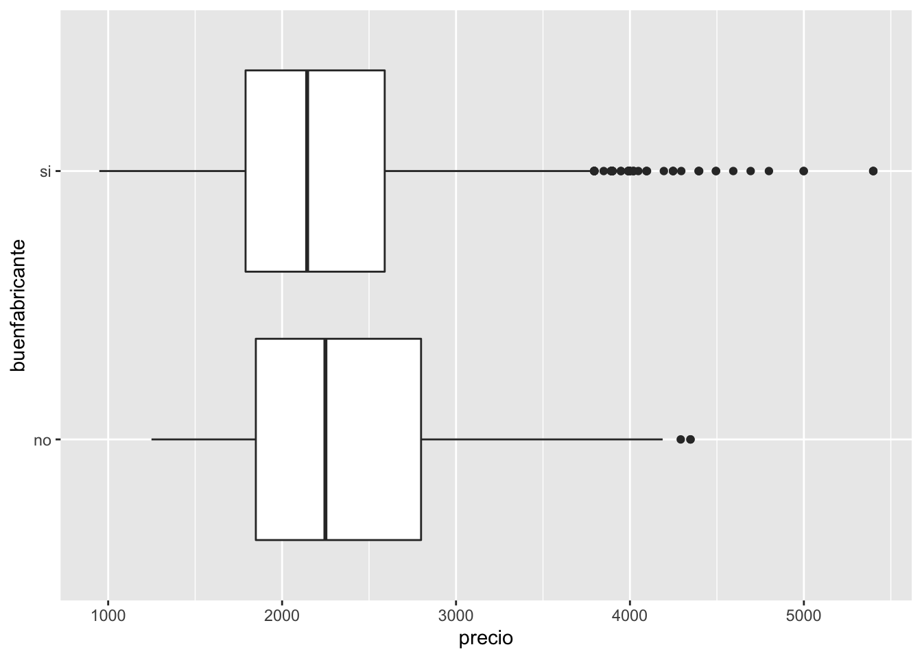
 $ buenfabricante: chr  "si" "si" "si" "no" ...
 $ numprecios    : num  94 94 94 94 94 94 94 94 94 94 ...
 $ numes.ene1993 : num  1 1 1 1 1 1 1 1 1 1 ...

Se realiza un resumen descriptivo de los datos:

Código

summary(datos)

     precio       velocidad            hd              ram        
 Min.   : 949   Min.   : 25.00   Min.   :  80.0   Min.   : 2.000  
 1st Qu.:1794   1st Qu.: 33.00   1st Qu.: 214.0   1st Qu.: 4.000  
 Median :2144   Median : 50.00   Median : 340.0   Median : 8.000  
 Mean   :2220   Mean   : 52.01   Mean   : 416.6   Mean   : 8.287  
 3rd Qu.:2595   3rd Qu.: 66.00   3rd Qu.: 528.0   3rd Qu.: 8.000  
 Max.   :5399   Max.   :100.00   Max.   :2100.0   Max.   :32.000  
    pantalla          cd               multi           buenfabricante    
 Min.   :14.00   Length:6259        Length:6259        Length:6259       
 1st Qu.:14.00   Class :character   Class :character   Class :character  
 Median :14.00   Mode  :character   Mode  :character   Mode  :character  
 Mean   :14.61                                                           
 3rd Qu.:15.00                                                           
 Max.   :17.00                                                           
   numprecios    numes.ene1993  
 Min.   : 39.0   Min.   : 1.00  
 1st Qu.:162.5   1st Qu.:10.00  
 Median :246.0   Median :16.00  
 Mean   :221.3   Mean   :15.93  
 3rd Qu.:275.0   3rd Qu.:21.50  
 Max.   :339.0   Max.   :35.00

Se construye un gráfico con ggplot2

Código

library(ggplot2)
library(dplyr)
datos %>% 
  ggplot(aes(x=buenfabricante,y=precio)) +
  geom_boxplot() +
  coord_flip()

Ejercicio 2

Creamos una matriz \(3 \times 3\) con elementos aleatorios:

Código

set.seed(1)
mat01 = matrix(rnorm(9),nrow=3,ncol=3)
mat01

           [,1]       [,2]      [,3]
[1,] -0.6264538  1.5952808 0.4874291
[2,]  0.1836433  0.3295078 0.7383247
[3,] -0.8356286 -0.8204684 0.5757814

Se calculan las máximos, mínimos y medias por columnas de esta matriz.

Procedimiento 1:

Código

s_maxC = rep(NA,ncol(mat01))
s_minC = rep(NA,ncol(mat01))
s_medC = rep(NA,ncol(mat01))

for (j in 1:ncol(mat01)) {
  s_maxC[j] = max(mat01[,j])
  s_minC[j] = min(mat01[,j])
  s_medC[j] = mean(mat01[,j],na.rm = T)
}

Código

s_maxC

[1] 0.1836433 1.5952808 0.7383247

Código

s_minC

[1] -0.8356286 -0.8204684  0.4874291

Código

s_medC

[1] -0.4261464  0.3681067  0.6005117

Procedimiento 2:

Código

(s_maxC02 = apply(mat01, 2, max))

[1] 0.1836433 1.5952808 0.7383247

Código

(s_minC02 = apply(mat01, 2, min))

[1] -0.8356286 -0.8204684  0.4874291

Código

(s_medC02 = apply(mat01, 2, mean,na.rm=T))

[1] -0.4261464  0.3681067  0.6005117

Procedimiento 3:

Código

colMeans(mat01)

[1] -0.4261464  0.3681067  0.6005117

Procedimiento 4:

Utilizando la filosofía “tidyverse”:

Código

library(tidyverse)
#library(tibble)
t_mat01 = as_tibble(mat01) # convertir a tibble
t_mat01

# A tibble: 3 × 3
      V1     V2    V3
   <dbl>  <dbl> <dbl>
1 -0.626  1.60  0.487
2  0.184  0.330 0.738
3 -0.836 -0.820 0.576

Código

t_res = 
t_mat01 %>% 
  summarise_all(list(max,min,mean)) %>% 
  as_vector() %>% 
  matrix(nrow = 3,dimnames = list(NULL,
                                 c("Max","Min","Medias"))) %>% 
  #as.data.frame()
  as_tibble()

t_res

# A tibble: 3 × 3
    Max    Min Medias
  <dbl>  <dbl>  <dbl>
1 0.184 -0.836 -0.426
2 1.60  -0.820  0.368
3 0.738  0.487  0.601

Ejercicio 3

La función se puede construir usando lo visto en el ejercicio 2:

Código

func_MMM = function(mat_input) {
(s_maxC02 = apply(mat_input, 2, max))
(s_minC02 = apply(mat_input, 2, min))
(s_medC02 = apply(mat_input, 2, mean,na.rm=T))
 l_res = list(Maximos = s_maxC02,
              Minimos = s_minC02,
              Medias = s_medC02)
 return(l_res)
}

Un ejemplo de uso:

Código

lr = func_MMM(mat01)
lr

$Maximos
[1] 0.1836433 1.5952808 0.7383247

$Minimos
[1] -0.8356286 -0.8204684  0.4874291

$Medias
[1] -0.4261464  0.3681067  0.6005117

Escribir la función en un fichero aparte e incorporarla en un documento R Markdown…